
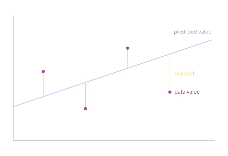
You fit a line through survey data, say ad spend against brand consideration, and the line never touches every point. The gaps are the part of the story your model did not tell, and they show whether it deserves your trust. They sit next to the correlation coefficient in our guide to correlation in survey research.
Key takeaways
- A residual is the observed value minus the value a model predicted, so in regression every data point has one residual, its vertical gap from the fitted line.
- Small, random residuals suggest the model fits, while a curve, a funnel or a drift in the residual plot shows that something is wrong.
- In the worked example, the residuals sum to zero, which checks the arithmetic but says nothing about how well the line fits.
- In a crosstab, a residual is observed minus expected count, and an adjusted residual beyond about 1.96 marks a cell that differs from independence.
- Do not delete a point just because its residual is large; check the record first and remove it only if it is an error.
What are residuals and how do you calculate them?
The formula is short:
residual = observed y - predicted y
The observed value comes from your data. The predicted value comes from the model, in simple regression the point on the fitted line directly above or below the observation. Every data point gets one residual.
A residual is not quite an error. The error is the gap between an observation and the true, unknowable relationship in the population. The residual is the gap to your estimated line, so it stands in for the error.
What does a worked example of residuals look like?
Five regions each report monthly ad spend (in thousands of dollars, x) and an average brand consideration score on a 0 to 10 scale (y).
First, fit the least-squares line. The mean of x is 3 and the mean of y is 4. The slope is the sum of (x minus 3) × (y minus 4) divided by the sum of (x minus 3) squared: (4 + 0 + 0 + 0 + 2) / (4 + 1 + 0 + 1 + 4) = 6 / 10 = 0.6.
The intercept is 4 - 0.6 × 3 = 2.2. So predicted y = 2.2 + 0.6 × x, and each residual follows.
| Region | Spend (x) | Observed y | Predicted y | Residual |
|---|---|---|---|---|
| A | 1 | 2 | 2.2 + 0.6 × 1 = 2.8 | 2 - 2.8 = -0.8 |
| B | 2 | 4 | 2.2 + 0.6 × 2 = 3.4 | 4 - 3.4 = +0.6 |
| C | 3 | 5 | 2.2 + 0.6 × 3 = 4.0 | 5 - 4.0 = +1.0 |
| D | 4 | 4 | 2.2 + 0.6 × 4 = 4.6 | 4 - 4.6 = -0.6 |
| E | 5 | 5 | 2.2 + 0.6 × 5 = 5.2 | 5 - 5.2 = -0.2 |
The residuals sum to zero: -0.8 + 0.6 + 1.0 - 0.6 - 0.2 = 0. That always happens with least squares when the model has an intercept, so it checks your arithmetic but says nothing about fit.
The squared residuals add up to 0.64 + 0.36 + 1.00 + 0.36 + 0.04 = 2.40. Dividing by the degrees of freedom (5 points minus 2 estimated parameters = 3) gives 0.80. Its square root, 0.89, is the typical miss in score points.
What do positive and negative residuals mean?
The sign gives the direction of the miss and the size gives how far off the model was, in the units of y.
- Positive residual: the observation is above the line, so the model underpredicted. Region C scored 1.0 point higher than its spend suggests.
- Negative residual: the observation is below the line, so the model overpredicted. Region A scored 0.8 points lower than predicted.
Treat either as a question, not an answer: a region that beats its spend might face a weaker competitor.
How do you read a residual plot?
A residual plot puts predicted values (or x) on the horizontal axis and residuals on the vertical axis, with a line at zero. If the model fits, the points form a shapeless band around it.
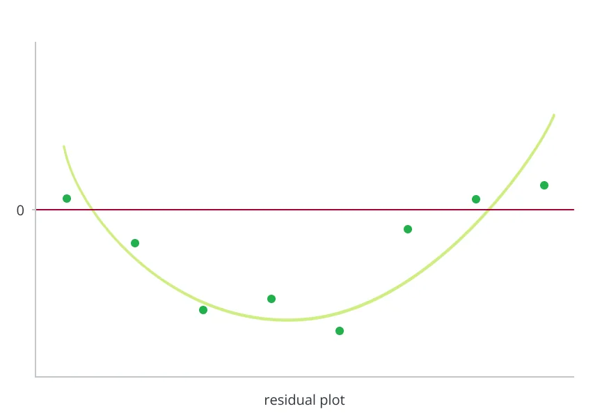
Patterns tell you what is wrong:
- Random band around zero: a straight-line model is reasonable.
- Curve or U shape: the relationship is not linear. Add a squared term or transform a variable.
- Funnel, with spread growing or shrinking: error size changes with the level of y. Transform y or use a method that allows unequal spread.
- Drift or runs in time order: observations are not independent.
- One point far from the rest: a possible outlier or data error. Check the record before changing anything.
Five points are enough to calculate residuals but not to judge a pattern. Plan on dozens of observations. For more on charting relationships, see visualizing correlations in survey analysis.
What are the different types of residuals?
Raw residuals are in the units of y, so a miss of 1.0 means different things on different scales. Rescaled versions fix that.
- Standardized residuals divide the raw residual by an estimate of the standard deviation of the errors. Here that is 0.89, so region C is 1.0 / 0.89 = 1.12 and region A is -0.8 / 0.89 = -0.89. Values beyond about 2 deserve a look.
- Studentized residuals also adjust for distance from the mean of x, because far-out points pull the line toward themselves.
- Deleted residuals come from fitting the model without that point. Their squares sum to the PRESS statistic, so the two are one idea.
- Deviance residuals are used for models such as logistic regression.
What are residuals in a crosstab and chi-square test?
Researchers meet residuals most often here. In a chi-square test of independence, the model is “the two questions are unrelated,” and each cell’s prediction is its expected count:
expected = row total × column total / grand total
The residual is observed minus expected. Take 200 respondents, 100 under 35 and 100 aged 35 or over, asked whether they are likely to buy.
| Group | Likely: observed | Likely: expected | Not likely: observed | Not likely: expected |
|---|---|---|---|---|
| Under 35 | 50 | 40 | 50 | 60 |
| 35 or over | 30 | 40 | 70 | 60 |
Likely buyers total 80 and the rest 120, so the expected count for under-35 and likely is 100 × 80 / 200 = 40. The raw residuals are +10, -10, -10, and +10. A gap of 10 means more against an expected 40 than 400, so we standardize.
- Standardized (Pearson) residual: (observed - expected) / square root of expected. For under-35 and likely, that is 10 / 6.32 = 1.58. For under-35 and not likely, it is -10 / 7.75 = -1.29.
- Adjusted standardized residual: divides by a smaller number that accounts for the row and column totals, here 3.46, so the first cell becomes 10 / 3.46 = 2.89. Every cell in this table has an absolute value of 2.89.
Adjusted residuals behave roughly like z-scores, so an absolute value above 1.96 marks a cell that differs from independence at the 95% level. The squared Pearson residuals add up to the chi-square statistic: 2.50 + 1.67 + 2.50 + 1.67 = 8.33, with 1 degree of freedom and p of about 0.004. In a larger table, adjusted residuals show which cells drive the result.
What are the most common mistakes with residuals?
- Judging fit from the correlation alone. Two datasets can share a correlation coefficient while one has random residuals and the other a clear curve. Look at the plot.
- Deleting points because their residuals are large. Check the record first. Remove a point only if it is an error.
- Reading a pattern into a handful of points. With ten observations, any shape can appear by chance.
- Comparing models by training residuals alone. A more complex model nearly always shrinks them. Compare on data the model has not seen.
- Reading raw differences in a crosstab. A gap of 10 against 400 expected is noise, and against 40 it is not. Use standardized residuals, and expect about 1 cell in 20 to pass 1.96 by chance.
How do you work with residuals in practice?
Halo Reports builds crosstabs and banner tables with weighting and significance testing, so you can see which cells differ from what chance alone would produce. For regression, most statistics packages can save residuals as a column you can plot.
If residuals cluster in one customer segment, the model is missing something about that group, and seeing what drives satisfaction and loyalty by segment is often the faster route to the answer. Next time you fit a model, plot the residuals before you report it. If you are still choosing predictors, a correlation matrix shows which variables move together. For wide, complex studies and global brand trackers, one governed platform for research teams keeps the data and the analysis together.